What is a Markov Chain?

A Markov Chain is a mathematical model describing transitions between states based on probabilities. Its defining property is that the future state depends only on the current state, not on past states.

Markov Property

The Markov Property is expressed mathematically as:

$$ P(X_{t+1} = s_j | X_t = s_i, X_{t-1}, …, X_0) = P(X_{t+1} = s_j | X_t = s_i) $$

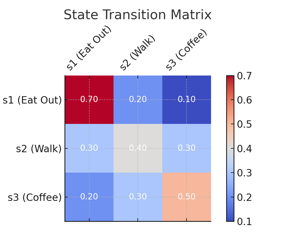
State Transition Probability Matrix

The state transitions in a Markov Chain are described by a state transition probability matrix, ( P ):

$$ P = \begin{bmatrix} 0.7 & 0.2 & 0.1 \ 0.3 & 0.4 & 0.3 \ 0.2 & 0.3 & 0.5 \end{bmatrix} $$

Each entry ( P(s_j|s_i) ) represents the probability of transitioning from state ( s_i ) to state ( s_j ). The rows of the matrix must sum to 1.

Visual Representation

Initial State Distribution

The initial state distribution is represented as a vector ( \pi ). For example:

$$ \pi^{(0)} = [1.0, 0.0, 0.0] $$

This means the system starts entirely in state ( s_1 ) (eating out).

Prediction Formula

To predict the state distribution at the next time step, use the formula:

$$ \pi^{(t+1)} = \pi^{(t)} \cdot P $$

Repeat this process iteratively to predict the distribution over multiple steps.

Practical Example: Deciding Daily Activities

Imagine you’re deciding what to do tomorrow:

1. Eat out (( s_1 )).
2. Go for a walk (( s_2 )).
3. Grab coffee (( s_3 )).

Based on your habits:

• If you eat out today, there’s a 70% chance you’ll eat out again tomorrow, 20% chance for a walk, and 10% chance for coffee.
• Similar transition probabilities apply for other states.

The state transition matrix ( P ) and initial state distribution ( \pi ) are as shown earlier. Let’s predict your activity distribution over the next 10 days.

Python Implementation

 1
 2
 3
 4
 5
 6
 7
 8
 9
10
11
12
13
14
15
16
17
18
19
20
21
22
23
24
25
26

import numpy as np

# Define the state transition matrix
P = np.array([
    [0.7, 0.2, 0.1],
    [0.3, 0.4, 0.3],
    [0.2, 0.3, 0.5]
])

# Define the initial state (starting with eating out)
initial_state = np.array([1.0, 0.0, 0.0])

# Function to predict future states
def predict_markov_chain(P, initial_state, steps):
    state = initial_state
    predictions = []
    for step in range(steps):
        state = np.dot(state, P)
        predictions.append(state)
        print(f"Step {step + 1}: {state}")
    return predictions

# Run the prediction for 10 steps
steps = 10
predicted_states = predict_markov_chain(P, initial_state, steps)
print("Predicted State Distribution After 10 Steps:", predicted_states[-1])

Example Output

Running the above code produces the following output:

1
2
3
4
5

Step 1: [0.7 0.2 0.1]
Step 2: [0.58 0.28 0.14]
Step 3: [0.494 0.318 0.188]
...
Step 10: [0.4 0.3 0.3]

By the 10th day, the probabilities stabilize at ( [0.4, 0.3, 0.3] ), indicating equal chances for eating out, walking, or grabbing coffee.

Conclusion

Markov Chains are versatile and easy to implement. Whether predicting daily decisions, modeling weather patterns, or generating text, they provide a powerful framework for understanding probabilistic systems.